Contents
- Introduction
- RISC-V register file
- Instructions
- Application Binary Interface (ABI)
- Instruction formats (encoding/decoding instructions)
- Register type (R-type) instruction format
- Four register type (R4-type) instruction format
- Immediate type (I-type) instruction format
- Store type (S-type) instruction format
- Branch type (B-type) instruction format
- Upper type (U-type) instruction format
- Jump type (J-type) instruction format
- Encoding example
- Decoding example
- Instruction pipeline
Introduction
We learned about the nomenclature of computer components, looked at the power of numbers in binary, and looked at digital logic and how we can put these together to produce a result. Now, we will see how we can put some of these together to process data. I use the term process because we can add, subtract, multiply, divide, and so forth.
The most basic central processing unit can be divided into three parts: (1) control unit, (2) arithmetic and logic unit (ALU), and (3) register file. The control unit is responsible for retrieving an instruction, decoding the operands by reading the registers or immediate value, and then sending it to the arithmetic logic unit (or floating-point unit).
All of the screenshots and information can be found in the riscv-spec PDF document in chapters 24 and 25.
RISC-V Register File
The RISC-V architecture in 64-bit mode has 32, 64-bit integer registers and 32, 64-bit floating point registers. All integer and floating point registers have two names–the register index, where integer registers are prefixed with an x, such as x0, x5, x10, etc. or the ABI name, which gives the purpose of the register, such as sp, a0, a1, t0, t1, and s0. In this course, we typically refer to a register by its ABI name.
A register is a small, 64-bit piece of memory built into a single core inside of the processor. Since RISC-V is a load/store architecture, any instruction requires the operands to be in registers before it can function. For example, if I want to add 3 and 2, the value 3 must be in one register, and the value 2 must be in another register before I execute the add instruction.
The following chart shows all of the registers inside of the RISC-V architecture.
| Name | ABI Mnemonic | Meaning | Preserved across calls? |
|---|---|---|---|
| x0 | zero | Zero | (Immutable) |
| x1 | ra | Return Address | No |
| x2 | sp | Stack Pointer | Yes |
| x3 | gp | Global Pointer | N/A |
| x4 | tp | Thread Pointer | N/A |
| x5 – x7 | t0 – t2 | Temporary Registers | No |
| x8 – x9 | s0 [fp] – s1 | Saved Registers | Yes |
| x10 – x11 | a0 – a1 | Argument and Return Registers | No |
| x12 – x17 | a2 – a7 | Argument Registers | No |
| x18 – x27 | s2 – s11 | Saved Registers | Yes |
| x28 – x31 | t3 – t6 | Temporary Registers | No |
| Name | ABI Mnemonic | Meaning | Preserved across calls? |
|---|---|---|---|
| f0 -f7 | ft0 – ft7 | Temporary Registers | No |
| f8 – f9 | fs0 – fs1 | Saved Registers | Yes |
| f10 – f11 | fa0 – fa1 | Argument and Return Registers | No |
| f12 – f17 | fa2 – fa7 | Argument Registers | No |
| f18 – f27 | fs2 – fs11 | Saved Registers | Yes |
| f28 – f31 | ft8 – ft11 | Temporary Registers | No |
The chart above shows 32 integer registers, denoted with an x0 through x31 and 32 floating point registers, denoted with an f0 through f31. These are the direct register names. All of the registers can be used as source and destination. However, in order for your code to work with C or C++, there must be a standard. This standard is called the application binary interface or ABI. The ABI we use in this class is RV64D, meaning that we have all of the integer instructions as well as the floating-point instructions.
All integer registers are 64 bits for a 64-bit machine. All floating point registers are 32 bits for a single-precision-only machine, or 64 bits for machines that support double precision. In this class, both the integer registers and floating point registers are 64 bits.
You will notice that a0, a1, fa0, and fa1 are used as both argument registers as well as return registers. For most cases, we will only use a0 or fa0 to return values.
The s0 register (x8) is the first saved register, but if a frame pointer is used to mark the stack, it becomes the fp (frame pointer) register.
Instructions
The way instructions are laid out, the register types, and the addressing modes of a CPU define its instruction set architecture or ISA.
Integer Instructions
| Instruction | Type | Description |
|---|---|---|
| addi rd, rs1, imm | I | rd = rs1 + imm |
| add rd, rs1, rs2 | R | rd = rs1 + rs2 |
| sub rd, rs1, rs2 | R | rd = rs1 – rs2 |
| mul rd, rs1, rs2 | R | rd = rs1 * rs2 |
| div rd, rs1, rs2 | R | rd = rs1 / rs2 |
| rem rd, rs1, rs2 | R | rd = rs1 % rs2 |
Logic Instructions
| Instruction | Type | Description |
|---|---|---|
| and rd, rs1, rs2 | R | rd = rs1 & rs2 |
| andi rd, rs1, imm | I | rd = rs1 & imm |
| or rd, rs1, rs2 | R | rd = rs1 | rs2 |
| ori rd, rs1, imm | I | rd = rs1 | imm |
| xor rd, rs1, rs2 | R | rd = rs1 ^ rs2 |
| xori rd, rs1, imm | I | rd = rs1 ^ imm |
| sll rd, rs1, rs2 | R | rd = rs1 << rs2 |
| slli rd, rs1, imm | I | rd = rs1 << imm |
| sra rd, rs1, rs2 | R | rd = (signed)rs1 >> rs2 |
| srai rd, rs1, imm | I | rd = (signed)rs1 >> imm |
| srl rd, rs1, rs2 | R | rd = (unsigned)rs1 >> rs2 |
| srli rd, rs1 imm | I | rd = (unsigned)rs1 >> imm |
Branch Instructions
| Instruction | Type | Description |
|---|---|---|
| beq rs1, rs2, label | B | goto label if rs1 == rs2 |
| bne rs1, rs2, label | B | goto label if rs1 != rs2 |
| blt rs1, rs2, label | B | goto label if rs1 < rs2 |
| bge rs1, rs2, label | B | goto label if rs1 >= rs2 |
| bltu rs1, rs2, label | B | goto label if rs1 < rs2 (unsigned) |
| bgeu rs1, rs2, label | B | goto label if rs1 >= rs2 (unsigned) |
Many of the branch instructions that you could think of, such as bgt, are pseudoinstructions, listed below. If a branch is not taken, meaning the condition is false, then the program counter is incremented by 4, which moves to the next instruction after the branch instruction.
Jump Instructions
| Instruction | Type | Description |
|---|---|---|
| jal rd, label | J | rd = pc + 4; pc = label |
| jalr ra, offset(rs1) | I | rd = pc + 4; pc = rs1 + sign_extend(offset) |
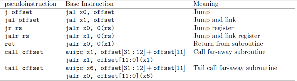
Jump instructions are typically used by programmers by using pseudo instructions, such as call (function call), j (unconditional jump), and ret (return from function call).
Memory Instructions
| Instruction | Type | Description |
|---|---|---|
| lb rd, offset(rs1) | I | rd = (char) *(rs1 + offset) |
| lbu rd, offset(rs1) | I | rd = (unsigned char) *(rs1 + offset) |
| lh rd, offset(rs1) | I | rd = (short) *(rs1 + offset) |
| lhu rd, offset(rs1) | I | rd = (unsigned short) *(rs1 + offset) |
| lw rd, offset(rs1) | I | rd = (int) *(rs1 + offset) |
| lwu rd, offset(rs1) | I | rd = (unsigned int) *(rs1 + offset) |
| ld rd, offset(rs1) | I | rd = (long) *(rs1 + offset) |
| sb rs2, offset(rs1) | S | (char) *(rs1 + offset) = rs2 |
| sh rs2, offset(rs1) | S | (short) *(rs1 + offset) = rs2 |
| sw rs2, offset(rs1) | S | (int) *(rs1 + offset) = rs2 |
| sd rs2, offset(rs1) | S | (long) *(rs1 + offset) = rs2 |
The important aspect is that the load instructions will sign-extend unless you use the load that ends with a u (unsigned). For example, lb sign extends whereas lbu zero-extends.
All offsets are absolute offsets. Unlike C++, assembly does not scale the offset by the data size (known as pointer arithmetic).
Floating-point Instructions
| Instruction | Description |
|---|---|
| flw rd, offset(rs1) | rd = (float) *(rs1 + offset) |
| fsw rs2, offset(rs1) | (float) *(rs1 + offset) = rs2 |
| fld rd, offset(rs1) | rd = (double) *(rs1 + offset) |
| fsd rs2, offset(rs1) | (double) *(rs1 + offset) = rs2 |
| fadd.s or fadd.d rd, rs1, rs2 | rd = rs1 + rs2 |
| fsub.s or fsub.d rd, rs1, rs2 | rd = rs1 – rs2 |
| fmul.s or fmul.d rd, rs1, rs2 | rd = rs1 * rs2 |
| fdiv.s or fdiv.d rd, rs1, rs2 | rd = rs1 / rs2 |
| fsqrt.s or fsqrt.d rd, rs1 | rd = \(\sqrt{\text{rs1}}\) |
| fcvt.dest.src rd, rs1 | Converts rs1 into rd (see notes below) |
| fmv.x.w or fmv.x.d rd, rs1 | Moves the value of a floating point register into an integer register. (see notes below) |
| fmv.w.x or fmv.d.x rd, rs1 | Moves the value of an integer register into a floating point register. (see notes below) |
| feq.s or feq.d rd, rs1, rs2 | rd = 1 if rs1 = rs2 or rd = 0 if rs1 != rs2 |
| flt.s or flt.d rd, rs1, rs2 | rd = 1 if rs1 < rs2 or rd = 0 if rs1 >= rs2 |
| fle.s or fle.d rd, rs1, rs2 | rd = 1 if rs1 <= rs2 or rd = 0 if rs1 > rs2 |
| fmadd.s or fmadd.d rd, rs1, rs2, rs3 | rd = (rs1 * rs2) + rs3 |
| fmsub.s or fmsub.d rd, rs1, rs2, rs3 | rd = (rs1 * rs2) – rs3 |
| fnmsub.s or fnmsub.d rd, rs1, rs2, rs3 | rd = -(rs1 * rs2) + rs3 |
| fnmadd.s or fnmadd.d rd, rs1, rs2, rs3 | rd = -(rs1 * rs2) – rs3 |
Floating point instructions are executed using the floating-point unit (FPU). So, integer registers must be translated into a floating point register by using the conversion instructions, such as fcvt. The fcvt instruction takes the data sizes separated by dots, such as: fcvt.s.w. This is in the format fcvt.dest.src. The source data type for fcvt.s.w is a word (int) and the destination is a single precision floating point (float). So, if I wanted to take a single-precision floating point number and convert it to an integer, I would use fcvt.w.s.
The fcvt instructions will convert to or from the IEEE-754 format into an integer format. However, we can move directly without any conversion using the fmv (floating point move). So, fmv.x.w will move an IEEE-754 floating point number into an integer register. Unless you know what to look for, the integer register will be nonsensical since it is still in IEEE-754 format.
The possibilities for a source or destination are: D (double precision), S (single precision), W (32-bit integer), or L (64-bit integer). You can convert between a double and a single precision value using fcvt.d.s which is from a single-precision floating point into a double-precision floating point.
Unlike the fcvt instruction, the fmv instruction performs no conversion. It is just a way to copy data from the ALU to the FPU or vice-versa.
Floating point comparisons are interesting, such as feq, flt, and fle. The destination register is an integer register, such as a0, t0, s0, etc. Then the operands, rs1 and rs2, are both floating point registers, such as fa0, ft0, or fs0. The integer register will be set to the value 1 if the comparison is true, or it will be set to the value 0 if the comparison is false.
The following shows how to branch comparing floating point numbers.
fle.s t0, fa0, fs0
bne t0, zero, yes_it_is_less_than
As you can see, we can use the bne or beq instruction with the zero operand since the only two values that t0 can be set in this case is either 0 or 1. So, if we want to test if the floating point comparison was true, we would use bne since t0 would be 1 and NOT EQUAL to 0 in this case. Otherwise, if we want to test if the floating point comparison was false, we would use beq, because recall that t0 would be 0 if fle.s is false.
There are only three comparison instruction formats (feq, fle, and flt). Everything else can be derived from that. For example, the pseudo-instruction fge will flip the operands and then use the fle instruction to compare them. For example,
fge.s t0, ta0, ts0
fle.s t0, ts0, ta0
The two instructions are identical. Notice that the operands are simply switched so we can use the real instruction. Even though we have three floating point comparison instructions, we can derive fne, fge, and fgt.
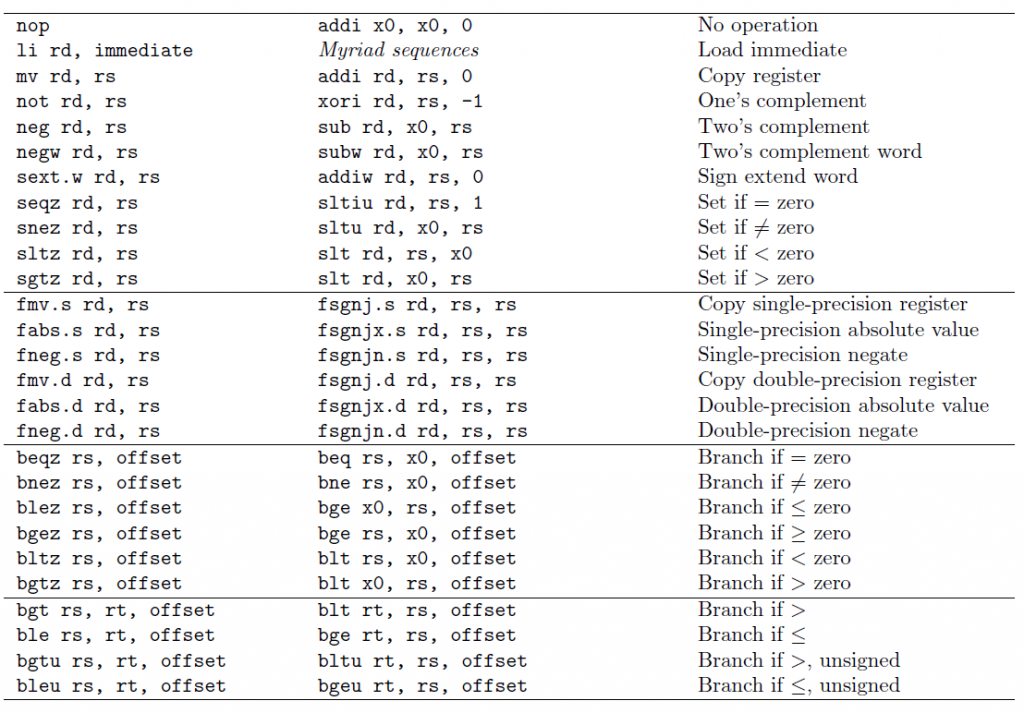
Pseudo Instructions
RISC-V is truly a reduced instruction set computer (RISC), so many of the common instructions have to use already existing instructions in a clever way. For example, there is no such thing as a pure jump instruction. Instead, we have the jump-and-link. However, we can emulate the jump instruction by using the zero register for rd. Recall that the zero register is hardwired to zero, so any writes to it are discarded.
To make the programmer’s job easier, the assembler, whose job it is to take assembly instructions and turn them into machine code, will allow the programmer to use fake instructions known as pseudo instructions.
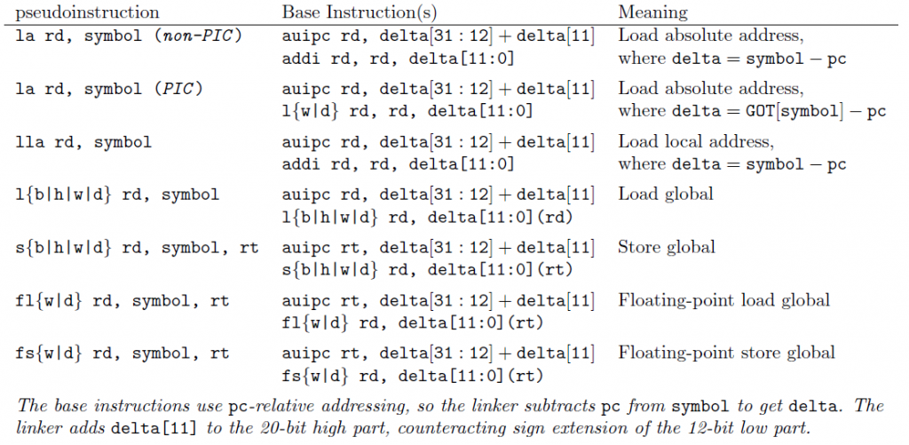
Recall that in the floating-point section, we also saw the pseudo instructions fgt (floating point greater than). We can also derive fge (floating point greater than or equal to). These pseudo instructions are available in RARS and in GAS (GNU assembler).
Application Binary Interface (ABI)
The application binary interface, or ABI for short, is a document that describes how registers will be used for a program. This allows all higher level code, such as C and C++, interact with other programs and even assembly language without having to translate.
In C or C++, the name of the function is the label name. However, to support overloading and namespaces, C++ will mangle the labels. Recall that in assembly, the labels must be unique, so overloading would not be possible. The mangled label contains the namespace, name of the function, and parameters. For example,
long add(long left, long right);
The C++ function above is actually labelled _Z3addll in assembly. I don’t expect you to know how to do this, and there is a way to turn it off using the extern “C” block.
extern "C" {
    long add(long left, long right);
}
Now that the prototype is in the extern "C" {} block, it will produce a label of add instead of _Z3addll.
The ABI register names have a specific purpose. For example, the a0 through a7 registers are the argument registers, t0 through t6 are temporary registers. There are other types of registers, such as the sp (stack pointer) and s0 – s11, which are the saved registers.
In order for our code to work correctly, we must follow these rules. If everyone follows these rules, we can coexist with C or C++ or even assembly language someone else already wrote.
The ABI is generally about functions. So, let’s take a C++ function as an example.
int func(int a, char b, short c, int *d);
The prototype above has three parts: (1) function name, (2) parameter list, and (3) return type. If we look at what this would look like in RISC-V assembly, we would see something like this:
a0 func(a0, a1, a2, a3);
.global func
func:
    # a0 = int a
    # a1 = char b
    # a2 = short c
    # a3 = int *d (this is a memory address)
    ret
As we can see above, we return a value by putting it into the register a0. This is why the chart shows a0 as both an argument register and the return register.
We can also see that the first parameter is a0, the second is a1, the third is a2, and the fourth is a3. No matter if the parameter is a char, int, short, or even a pointer, it still goes into the register–we just use a portion of the register instead of the full thing. The only time this changes is if we use a floating point register, such as fa0.
If we mix the two, then we use the first available register. For example, if we have an integer, a float, a double, and another integer, then the first integer would be put in a0, the float in fa0, and the double in fa1, and the second integer into a1.
Executable Sections
Recall that the compiler produces an assembly file, the assembler produces an object file, and the linker produces the executable. Each executable contains certain sections that store all of the information needed to run a program. These include four sections: (1) .rodata (read only data), (2) .data, (3) .bss (block stack section), and (4) .text (code section).
CPU instructions, the actual code, goes into the .text section. This section can then be given permission to execute CPU instructions. The rodata section contains global constants. The data section contains global, initialized variables. The BSS section contains global, uninitialized variables.
You may be wondering where local variables and constants go. Those go onto the stack, which we explore below.
Stack Pointer (sp)
The final special register we will talk about is called the stack pointer. Local variables are stored on the stack, which is a contiguous piece of memory that grows from high memory to low memory addresses. The stack pointer initially points to the very bottom of the stack. So, if we want to allocate space on the stack, we subtract the number of bytes we want from the stack pointer, and to deallocate space, we add the same number back to the stack pointer. The stack pointer must be aligned to 16 bytes. This means that the stack pointer must always be a multiple of 16. So, if we need 3 bytes from the stack, we must subtract 16 bytes. If we need 12 bytes from the stack, we must subtract 16. Alignment is used to make the memory controller’s job easier.
The following shows how to allocate enough bytes for an integer and three chars, which is a total of 7 bytes. So, we need to round 7 up to the nearest 16, which is 16 itself.
# Allocate by subtracting
addi sp, sp, -16
# integer at bytes sp+0, sp+1, sp+2, and sp+3
# char at byte sp+4
# char at byte sp+5
# char at byte sp+6
# bytes 7, 8, 9, 10, 11, 12, 13, 14, 15 are all empty.

# Deallocate by adding
addi sp, sp, 16
Stack Pointer Alignment
The stack pointer must always be a multiple of 16 bytes. This complicates things when we have an unknown number of values. However, we can use arithmetic and logical operators to align up and align down.
Stack Frames
A stack frame refers to a range of the overall stack space allocated to a particular routine or function. To ensure that functions do not destroy each others’ data, each function allocates a stack frame.
When a function starts, such as int main, the frame has not been moved. Recall that if I need to allocate memory, I subtract from the stack pointer. The memory between the original location of the stack pointer and the new location of the stack pointer is the stack frame.
Recall that the initial portion of a function is a prologue, which sets up the stack frame and saves all required registers before the function actually starts. Then, the function performs its operation. Finally, an epilogue cleans up and restores what was saved in the prologue. This is called a call stack.
The stack pointer register, sp, marks the start of a function’s stack space. There is another register called the frame pointer, fp, that marks the end of a function’s stack space, which is the original location of the stack pointer. The following assembly code shows a function’s prologue and setting of the stack and frame pointers.
add:
    addi sp, sp, -16    # Move the stack pointer
    sd   fp, 0(sp)      # Store the old frame pointer
    addi fp, sp, 16     # Mark the end of the stack space with the frame pointer

    sd   ra, 8(sp)      # We use positive numbers for the stack pointer
    # ... or ...
    sd   ra, -8(fp)     # or negative numbers for the frame pointer

    # ...

    ld   ra, 8(sp)
    ld   fp, 0(sp)      # Restore old frame pointer
    addi sp, sp, 16     # Move stack pointer back

    ret
By abiding by the stack frame rules, functions can make sure they don’t corrupt the data of the other functions.

Stack Security
However, recall that the stack is still just a contiguous piece of memory, and we can load or store any memory address we want. In fact, the way this memory is laid out is a cause of many security concerns.
For example, if I was somehow able to manipulate the offset of a pointer, I could potentially read values not intended for me. If this is done on accident, it is called stack squashing or smashing.
For example, the C++ code is completely legit, but as you can see, we can observe variable that aren’t ours.
#include <iostream>
using namespace std;

void squash() {
    double p[1];
    p[4] = 5.7;
}

int main() {
    double j = 22.5;
    cout << j << '\n';
    squash();
    cout << j << '\n';
}
The code above prints 22.5 before the squash call and 5.7 after the squash call, even though we never actually change the value of j, but since j is on the stack, we were able to move our pointer around to find it and reset it.
The reason I subscripted 4 from the array is because the squash function allocates 32 bytes from the stack, which means it subtracts 32 from the stack pointer. So, since doubles are 8 bytes, \(8\times 4=32~\text{bytes}\). So, now we are dereferencing the stack pointer’s original spot, which belongs to int main(), and, more specifically, is the variable double j.
Argument Registers (a0 – a7, fa0 – fa7)
The argument registers are used for three purposes: (1) as arguments to a function call, (2) a0 is also the return value register, and (3) any argument register not being used for arguments or return values are extra temporary registers.
The argument registers are ordered, meaning the first argument to a function is always a0, the second is always a1, and so forth. Any argument after a7 is put on the stack, but we will not cover this scenario in this class. You may not just simply choose any argument register as arguments to a function call. However, you are permitted to use any argument register if it is not being used as the return register or any argument register.
A system call can be made by using the ecall instruction (environment call). However, we must use a particular argument register so that the operating system knows which call we want (which are all based off of a table of numbers). In this case, the a7 register is used to store the system call number, and then the arguments to the system call goes into a0 through a6. Obviously, there is one fewer argument register for system calls than there is for regular function calls.
The floating point values use the same registers, except they are prefixed with an f for floating point, such as fa0, fa1, fa2, …, fa7.
For example, the following function prototype MUST use the argument registers identified below.
long myfunc(int a, int b, int c, float d);
// uses the following registers
a0 myfunc(a0, a1, a2, fa0);
Temporary Registers (t0 – t6)
Temporary registers are just that–temporary. After you make a function call ALL temporary registers must be considered to no longer have the value you put in there. No matter whether it actually does is immaterial. You must act as if the temporary registers have destroyed its values. If you want the value in a temporary register to remain after a function call, you must either save it on the stack or put it in a saved register. However, using a saved register requires you to save the old value prior to using it.
The following example shows saving the value of a temporary register, calling a function, and then restoring its value. Recall that the stack must always be a multiple of 16!
.global main
main:
   addi   sp, sp, -16
   sd     t0, 0(sp)
   sd     t1, 8(sp)
   call   some_function
   ld     t0, 0(sp)
   ld     t1, 8(sp)
   # Use t0 and t1 here as if nothing happened.
   addi   sp, sp, 16
Saved Registers (s0 – s11)
There is a difference between caller saved and callee saved registers. Any caller saved register is free to be used without regard of the previous value. However, a function may use a callee saved register provided it restores the original value of the register before the function returns. In other words, if you use any register s0 through s15, you must return it back the same way you found it. Typically, you will use the stack to store the original value and load back the original value before you return.
myfunc:
    # We are going to use the s0 and s1 registers, so we need
    # 8 bytes for the s0 register and 8 for the s1 register
    # so 16 total.
    addi   sp, sp, -16
    sd     s0, 0(sp)
    sd     s1, 8(sp)
    # Now that s0 and s1 are saved, they may be used
    # for any purpose.

    # Now, before we return, restore the original values
    # into s0 and s1
    ld     s0, 0(sp)
    ld     s1, 8(sp)
    addi   sp, sp, 16

    # s0 and s1 are good to go! We're OK to return
    ret
Notice above that I always use sd and ld when saving or restoring saved registers. This is because we want to save the entire register, since we don’t know how much of the register is actually being used. So, to be safe, we save the entire register. It may even contain junk, we don’t care, we just have to save that junk, use the saved register, and then restore that junk. We cannot differentiate good data from junk, so we always assume it is good data.
Endianness
The architecture needs to decide how it will store multiple bytes into memory. It can do this one of two ways: (1) store the least significant byte first (called little endian) or (2) store the most significant byte first (called big endian). The following diagram depicts the difference between little endian and big endian:
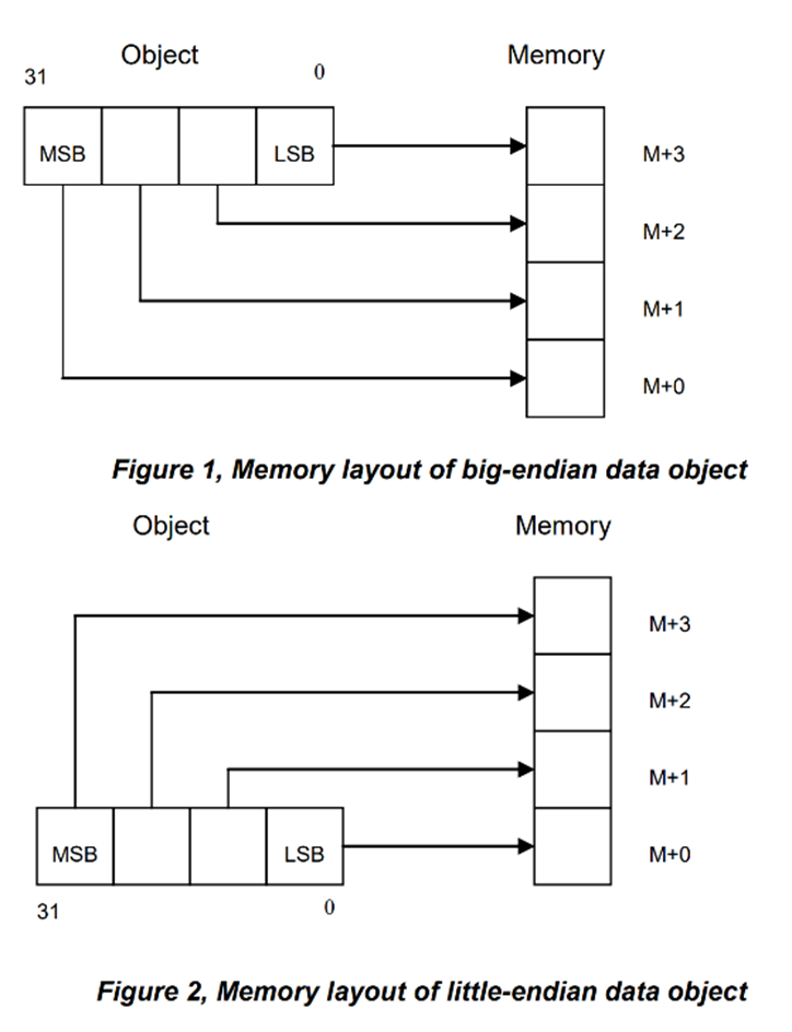
You can see from above, the least significant byte (LSB) is stored at memory offset 0 in a little endian system, and the most significant byte (MSB) is stored at memory offset 0 in a big endian system.
Endianness only matters with multiple byte data types, such as a short (2 bytes), int (4 bytes), long (8 bytes), or even a float (4 bytes) or double (8 bytes).
The following code depicts why this is important.
unsigned int value = 0xdeadbeef;
unsigned char *p = (unsigned char *)&value;

printf("%08x\n", value);
printf("%02x %02x %02x %02x\n", p[0], p[1], p[2], p[3]);
On a little endian system, the following is printed to the screen.
deadbeef
ef be ad de
On a big endian system, the following is printed to the screen.
deadbeef
de ad be ef
In some circumstances, you will need to know the endianness. For example, if a file is in big-endian format, it must be converted to the architecture’s endianness. Another example is through WiFi or Ethernet. The data sent and received through WiFi and Ethernet is sent in big endian.
Most architectures we see now are little endian, including RISC-V, ARM, and Intel/AMD computers.
Memory Structures (N.O.S.)
An array and a structure are two of the several ways C/C++ organizes memory so you, the programmer, may use it. To optimize the speed of reading and writing memory, C/C++ manages how an array or structure is organized.
Arrays
Arrays are just multiple, contiguous sections of memory of the same data type. This makes our job easy because C/C++ just multiplies the size of the data type with the number of elements to determine how much memory needs to be allocated. The following figure depicts an array of four integers.
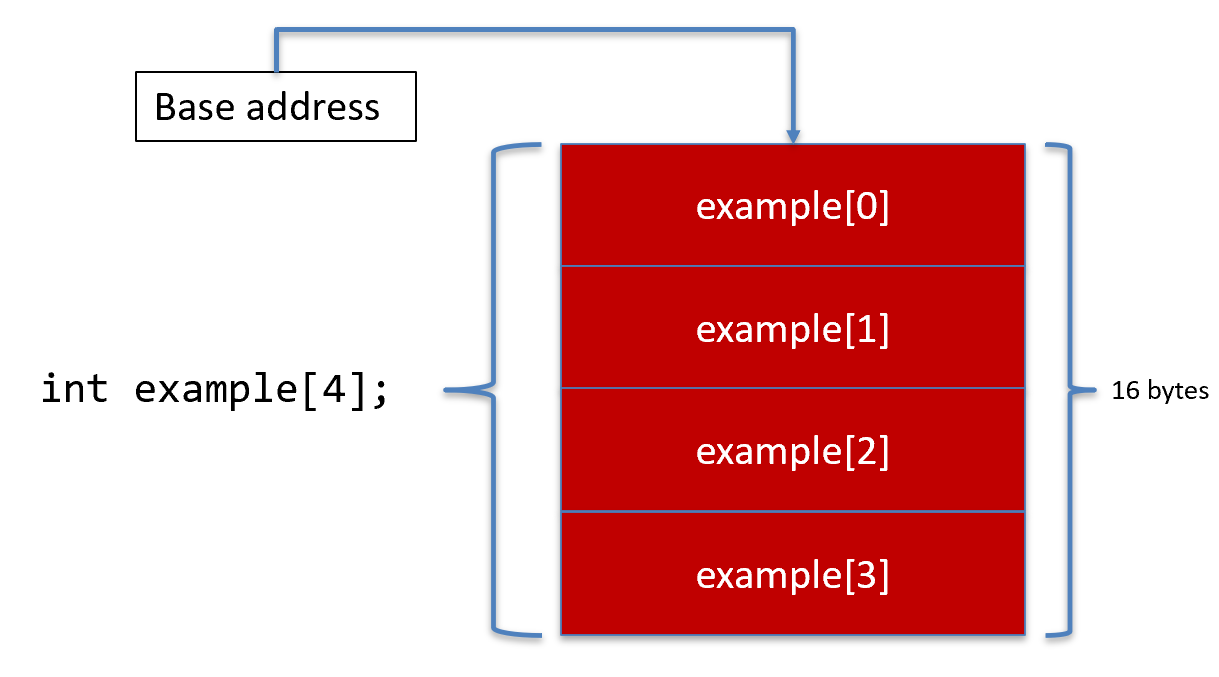
An array is actually a pointer. Recall that pointers store memory addresses. The memory address that an array stores is the first byte of the first element. This is called the base address.
Since each element is exactly the same size, and since the array is in contiguous memory, each element’s memory address is determined by simple arithmetic.
Element Address = Base Address + Index * Size
The base address is the first byte of the first element, and the index is the index you put in the subscript operator (e.g, example[2]). So, if C/C++ put the first byte of the first element to memory address 0x1000, then to get example[3], we use the formula: 0x1000 + 3 * 4 = 0x1000 + 12 = 0x100c. Therefore, C/C++ knows to dereference the 4-byte value at memory address 0x100c, which will get example[3].
Structures
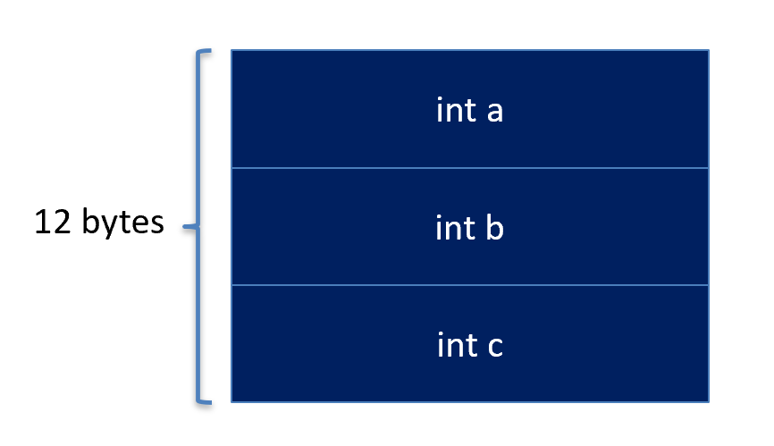
A structure is just a way to put fields together in memory. Given the following structure,
struct MyStruct {
   int a;
   int b;
   int c;
};
The C/C++ compiler will organize into memory as follows:
Unlike arrays, structures may contain different data types, and hence, different sizes. However, just like arrays, a structure is actually stored as the first byte of the first element. So, C/C++ still needs to use some sort of formula to determine how to get to each and every field in a structure. This is done through a Name, Offset, Size (NOS) table. As the name implies, the table contains three columns: (1) the name of the field, (2) the number of bytes from the beginning of the structure, and (3) the size of the field.
The C/C++ compiler optimizes how structures are stored by adding bytes that are not associated with any fields. These extra bytes are called padding, and they take up extra space to speed up memory reads and writes.
The rules of padding are as follows:
- The offset of each field must satisfy the following equation: offset % field size == 0.
- The last field is padded by rounding up to a multiple of the largest data type in the entire structure.
The following depicts a structure of differing data types and how padding will be added to the structure.
struct MyStruct {
    char a;
    short b;
    int c;
};
The structure above produces the following memory format.

How did C/C++ produce that structure? Well, we can design a NOS table using the rules above.
| Name | Offset | Size |
|---|---|---|
| char a | 0 | 1 |
| short b | 2 | 2 |
| int c | 4 | 4 |
The first field of every structure is at offset 0 because the structure is referenced by the first byte of the first field, much like an array. We then have to apply the rules to determine the next offsets.
So, if char a is occupying byte 0, the next byte we have available is byte 1. However, 1 % 2 != 0, which violates the first rule. So, we keep adding padding bytes until x % 2 == 0. So, 1 goes to 2 % 2 == 0, which is why short b starts at offset 2. So, now short b occupies bytes 2 and 3, so the next byte available is 4, and 4 % 4 == 0, so we can pack int c right after short b. We also need to consider the final padding. The next byte available is 8, and the largest data size is 4. 8 % 4 == 0, so we do not need to add any padding byte. Therefore, we know that this structure is exactly 8 bytes.
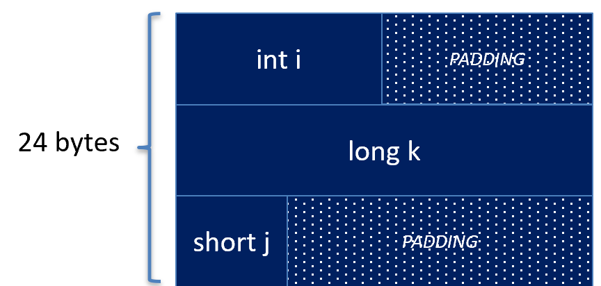
Unfortunately, not all structures are this convenient. Since any structure may be put into an array, we may need to add padding bytes at the end of the structure instead of in-between the fields of a structure. The following structure depicts one that needs ending padding bytes.
struct MyStruct {
    int i;
    long k;
    short j;
};
The structure above has the following NOS table.
| Name | Offset | Size |
|---|---|---|
| int i | 0 | 4 |
| long k | 8 | 8 |
| short j | 16 | 2 |
As always, the first field takes offset 0. So, the integer above takes bytes 0, 1, 2, and 3. The next available byte we have is 4, but 4 % 8 != 0, so we need to pad it to the next multiple of 8, which is 8. So, 4 bytes of padding are placed in-between int i and long k. Now, bytes 8, 9, 10, 11, 12, 13, 14, and 15 are occupied by long k. So, the next available byte is 16, and 16 % 2 == 0, so the short j may be stored at offset 16. Now, the short takes bytes 16 and 17. However, now we need to determine the padding at the end. The largest data size is the long at 8 bytes, and the next byte available is 18, but 18 % 8 != 0, so we need to pad up to the nearest multiple of 8, which is 24. So, bytes 18, 19, 20, 21, 22, and 23 are occupied by padding bytes.
The NOS table then forms the following structure in memory.
Padding is a pain to deal with, but it improves the performance of the memory controller, and for some architectures, it is a necessity. Some architectures will not allow you to LOAD or STORE a memory address that isn’t a multiple of the data size. Fortunately, these architectures are getting harder to find nowadays.
Returning Structures
As you have seen above, the a0 register returns the value, however, recall that no register can store a structure. Instead, structures are formed in memory. In C, you could not return a structure from a function, and instead, you would pass a pointer for the function to write into the structure. However, C++ now allows this. For example,
struct MyStruct {
    int a;
    int b;
};
MyStruct doit(int x, int y);
The doit function above returns a MyStruct. However, this cannot actually happen. Instead, C++ will place the memory address of the returned structure into the return register a0 before the function call. So, given the code above, it would in reality look like the following in assembly:
void doit(MyStruct &s, int x, int y);
So, above, the value of int x gets placed into a1, the value of int y gets placed into a2, and finally, the memory address of the MyStruct structure gets stored into a0. (Note: there are different rules based on the size of the structure….see below).
Small Structures
Structures that can be fit into one or two 8-byte registers will be stored into a0 and a1. For example, the given structure is passed in a0 and a1.
struct MyStruct {
    int a;
    int b;
    int c;
    int d;
};
In this case, a0 will contain int b in the upper 4 bytes and int a in the lower 4 bytes (little end first) and a1 will contain int d in the upper 4 bytes and int c in the lower 4 bytes.
Bottom line: if your structure is <= 16 bytes, the procedures change.
Returning Small Structures
The same thing about passing structures occurs when returning structures <= 16 bytes. 16 bytes of data can be returned in a0 (first 8 bytes) and a1 (second 8 bytes). Taking our structure from before, we can return a MyStruct using the following prototype:
struct MyStruct {
    int a, b, c, d;
};

extern "C" {
    MyStruct mystruct(int a, int b, int c, int d);
}

int main() {
    MyStruct ms = mystruct(1, 2, 3, 4);
}
Now, to return a MyStruct with the values 1, 2, 3, and 4, we need to store 1 in the lower four bytes of a0, which corresponds with int a, we store 2 in the upper four bytes of a0, which corresponds with int b, we store 3 in the lower four bytes of a1, which corresponds with int c, and we store 4 in the upper four bytes of a1, which corresponds with int d.
Our assembly would look as follows:
.section .text
.global mystruct
mystruct:
    slli    t0, a1, 32   # Shift int b up 4 bytes.
    or      a0, t0, a0   # Move int a to the bottom 4 bytes.

    slli    t1, a3, 32   # Shift int d up 4 bytes.
    or      a1, t1, a2   # Move int c to the bottom 4 bytes.

    ret
As you can see a0, a1, a2, and a3 contain the four parameters int a, int b, int c, and int d. We then shift them into place to return them in a0 and a1.
Floating Point Small Structures
If a structure only contains one or two floating point reals, either float or double, then these are passed as fa0 and fa1. If a single integer (char, short, int, or long) and a single float (float or double) are in a structure, then the floating-point is passed in fa0, and the single integer is passed in a0, regardless of the order in the structure.
Instruction Formats (encoding/decoding)
An instruction is simply a list of 0s and 1s that contain information needed to tell the CPU what instruction you want to execute and the parameters for that instruction. In RISC-V, each instruction is 32 bits. RISC-V also contains a compressed format that allows for 16-bit instructions. This means that all the information to instruct the CPU needs to fit within 32 bits.
The portion of the instruction that tells the CPU what instruction to execute is known as the operation code (opcode). In RISC-V, this is the last 7 bits of the instruction, and it tells the CPU whether to add, subtract, multiply, jump, branch, and so forth. For all 32 bit instructions, the last two bits of the 7-bit opcode are always \(11_2\). So, in all, there is a 5-bit opcode.
The table of opcodes that RISC-V understands is listed below. An opcode might not narrow down to a single instruction, instead, it might narrow down to a smaller subset of instructions. In the latter case, it requires a subopcode to further narrow down the instruction.
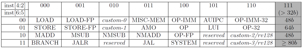
As you can see in the figure above, the three-bit column is made up of bits 4, 3, and 2 of the instruction, whereas the two-bit row is made up of bits 6 and 5. We talked about a multiplexor in the digital logic portion, and as you can see, the 5-bit opcode above is the selector for a multiplexor.
If we delve deeper into an instruction, we can see that it can contain additional information, such as the source operands and where we want the CPU to store the result. There are several different types of instructions, however each instruction is still 32 bits. The type of instruction just distinguishes how the bits will be interpreted.
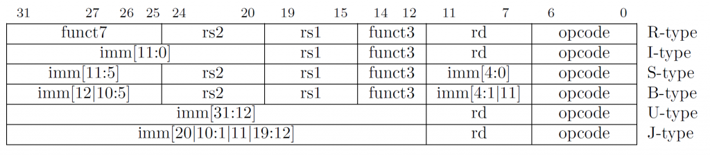
Register Type (R-type) Instruction Format
As you can see above, the opcode is always bits 0 through 6 (7 bits). The R-type stands for register type, meaning that the source operands are rs1 (register source 1) and rs2 (register source 2) and the destination is denoted by rd (register destination). We also talked about subopcodes, which we can see in the R-type with funct3, which is a 3-bit extenstion to the opcode, and funct7, which is a 7-bit extension to the opcode. When combined, this forms a 17-bit opcode that tells the CPU what instruction to run.
Four Register Type (R4-type) Instruction Format
This instruction format is mainly used for floating point instructions that requires four different registers encoded in one instruction.

You can see that we need this when encoding one destination and three source registers, such as the instruction fmadd.s rd, rs1, rs2, rs3. This performs the following: rd = rs1 * rs2 + rs3.
Immediate Type (I-type) Instruction Format
An immediate type uses one register-based source operand (rs1), but the second operand is known as an immediate, which is a small integer literally encoded in the instruction itself. If you remember, all registers are 64-bits for RISC-V64, but for the I-type instruction, we have a 12-bit immediate from bits 31 through 20. This means we will need to widen the 12-bit immediate to a 64-bit immediate. The instruction we choose will determine whether we sign-extend or zero-extend.
The LOAD set of instructions are also I-type instructions. They have the following format:
l<b[u]|h[u]|w[u]|d> rd, signed_imm(rs1)
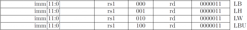
Since the immediates of all LOAD instructions are signed, you must sign-extend the immediate. This immediate is directly added to the value rs1 to form an effective memory address. This then becomes the memory address requested by the memory controller.
Do NOT confuse LBU and LB. They both still have a signed immediate. The difference is that LBU will zero-extend the value returned by the memory controller, whereas LB will sign-extend the value returned by the memory controller.
You can also see that all of the LOAD instructions have the same opcode. So, the funct3 becomes the data size and signedness. The leftmost bit of funct3 is 0 if the instruction sign extends, and it will be 1 if the instruction zero extends. The lower (rightmost) two bits describes the number of bytes to load. \(00_2\) is 1 byte, \(01_2\) is 2 bytes, \(10_2\) is four bytes, and \(11_2\) is 8 bytes.
Store Type (S-type) Instruction Format

The instruction format above has the STORE opcode, so the store selection (store byte, store half, store word, store doubleword) is all based on the 3-bit subopcode funct3. The important part about this instruction format is to differentiate between register source 1 (rs1) and register source 2 (rs2).
The store has a format like the following.
sh a0, -4(sp) # sh src, offset(base)
The instruction above will take the halfword (16 bits) from the register a0 and store it in the memory location pointed to by sp + -4. You can see from the instruction above that the rs2 is the source register. In other words, it’s the value you want to store into memory. Secondly, you can see that the rs1 register is the base register, which is the memory address where we want to store the value.
Lastly, the offset is a 12-bit value, but in the store format, it is split between bits 31-25 and bits 11-7.

You can see from the SB, SH, and SW instructions above, that the opcode is the same, but the subopcode (funct3) determines the number of bytes that will be stored.
Branch Type (B-type) Instruction Format
A branch instruction is an instruction that compares the values in two registers and jumps to a section of code based on the condition. For example, BNE stands for “branch if not equal”. So, in this case, we need two registers to compare, a condition code, and an offset to go to. The immediate field in the encoded instruction is the signed-offset.
The important part about a branch instruction is that the offset is PC-relative. This means that it is a signed-offset that is added to the program counter (PC). Recall that the program counter contains the address of the instruction the CPU will execute.

So, in this instruction, we can see the condition code is encoded in the funct3 field, which is a three-bit extended opcode. We can also see the immediate is somewhat odd. Notice that bit 0 is not stored in the immediate. This means that all numbers have to be a multiple of 2 to branch to it. The reason is because the smallest instruction is 2 bytes for compressed instructions. Therefore, all instructions have a 0 in the one’s digit.
When a branch instruction is “taken”, meaning the condition is true, then the immediate is added to the program counter (PC). Otherwise, the program counter moves to the very next instruction.
Upper Type (U-type) Instruction Format
Since we can only encode an instruction using a maximum of 32 bits, it is sometimes important that we use two instructions to write a full 32-bit or 64-bit value into a register. We can combine an upper-immediate, which requires a larger immediate space to store the value.

Notice that the immediate only stores bits 31 through 12. These instructions will set bits 31 through 12 of the register to the given immediate. Recall that with immediate-type instructions, the lower immediate is 12 bits. So, we can store the upper 20 bits using load upper immediate (lui), and then the lower 12 bits using an instruction such as addi.
Jump Type (J-type) Instruction Format
We saw that the branch instructions are PC-relative, but two registers eat up some of the offset. With the jump instructions, we still have a PC-relative, signed offset, but now we have more space. In fact, we now have 20 bits instead of 12.

Notice that most of the instruction encoding is dedicated to storing the lower 20 bits, except the one’s place. Again, just like with the branch instruction, the immediate is at least a multiple of 2 since all instructions are at least 2 bytes.
Encoding Instructions Example
Encoding is also known as “assembling”, where human-readable instructions are turned into 0s and 1s.
sh a0, -8(sp)
The registers a0 and sp are called ABI-format registers. These have a number between 0-31, which we can see at the register chart. The a0 register is x10 and the sp register is x2, so 10 (or 0b01010) and 2 (or 0b00010).
We then look at the SH (store halfword) instruction:

We need to fill in imm, rs2, and rs1. rs2 is the “source register”, which in this case is the A0 register, which we converted to X10. The rs1 register is the “base register”, or the base of the memory address, which is the SP register or X2. The immediate is broken into two pieces, bits 11 through 5 are on the left and bits 4 through 0 are on the right. So, we know this will be a 12-bit immediate (11-0). Our immediate (offset) is -8, so we need to write -8 using 12 bits:
-8 = ~(8) + 1
-8 = ~0b0000_0000_1000 + 1
-8 = 0b1111_1111_1000
The upper 7 bits will be 0b1111_111, and the lower 5 bits will be 0b1_1000.
Now to convert our registers. Each register field (rs2 and rs1) use 5 bits, which allows numbers from 0 – 31. So, X10 using 5 bits is 0b01010 and X2 using 5 bits is 0b00010.
Now we have all of the pieces of information we need to create a full 32-bit instruction.
imm[11:5] = 0b1111_111
rs2       = 0b0_1010
rs1       = 0b0_0010
func3     = 0b001
imm[4:0]  = 0b1_1000
opcode    = 0b010_0011

Put it all together:
1111_111  0_1010  0_0010  001  1_1000  010_0011

Group into fours:
1111 1110 1010 0001 0001 1100 0010 0011

Convert to hex
F    E    A    1    1    C    2    3

So,
sh  a0, -8(sp)

is,
0xFEA1_1C23
Decoding Instructions Example
Decoding an instruction is also called “disassembling”, where we convert the 0s and 1s into the assembly instructions we can read.
Convert: 0xFF01_8413
The first thing we need to do is to convert to binary so we can look at the 7-bit opcode:
0xFF01_8413 = 0b1111_1111_0000_0001_1000_0100_0[001_0011]
Opcode = 0b001_0011
We know this is a 32-bit instruction since the last two bits of the opcode are 0b11. Now, we need to look at the chart to see which type of instruction this is.
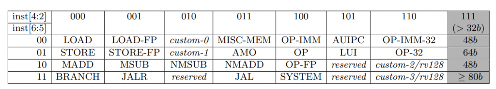
Our bits 6:5 are 0b00 and our bits 4:2 are 0b100. The last two bits are cut off since this chart is only for opcodes with the last two bits of 0b11.
Looking at the chart, we can see that column 0b100 and row 0b00 gives us the OP-IMM, meaning it is an operation that decodes an immediate, such as xori, addi, ori, srli, and so forth. If this was an R-type, it would simply by the OP category, and lastly OP-FP means “floating point”, such as fadd, fmul, etc.
Now that we know this is an immediate, we can decode the portions of an I-type instruction:
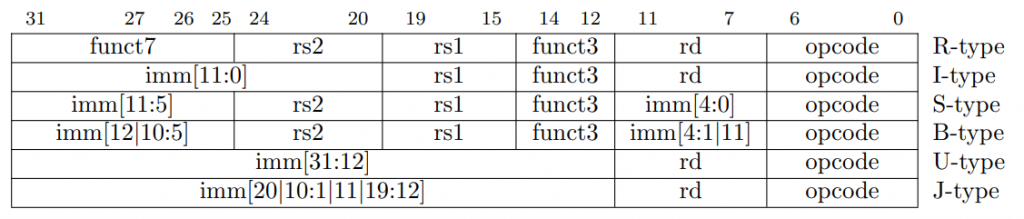
The instruction formats table above has the I-type, which means we need to decode: imm[11:0], rs1, funct3, rd, and we already have the opcode, so getting our original number:
0xFF01_8413 = 0b1111_1111_0000_0001_1000_0100_0001_0011
0b[1111_1111_0000] [00011] [000]   [01000] [001_0011]
    imm[11:0]        rs1   funct3    rd     opcode
imm[11:0] means a 12-bit immediate value, rs1 means the “source” register, and rd means the “destination” register. We can now convert the values:
imm[11:0] = 0b1111_1111_0000 (sign bit is 1)
-(~0b1111_1111_0000 + 1) = -(0b0000_0001_0000) = -16.

rs1 = 0b00011 = x3 = gp
rd  = 0b01000 = x8 = s0
Now we have to look at the opcode and funct3 to determine which instruction this is:

So, our funct3 is 000, and our opcode is 001_0011, which matches the ADDI instruction. Now, to put it all together, we get:
addi s0, gp, -16
Instruction Pipeline
To execute an instruction, several things need to take place. An oscillator is used as a clock to keep moving the program counter. So, for a single-cycle CPU, the instruction must be fetched, decoded, executed, and the result must be stored all within one cycle of the clock.
Instead of using a single-cycle, we can pipeline, which essentially splits these into five stages. The five stages are (in order): (1) instruction fetch (IF), (2) instruction decode (ID), (3) execute (EXE), (4) memory (MEM), and (5) write-back (WB). This five stage pipeline is known as the 5-stage RISC pipeline. This is mainly an academic pipeline, as many pipelines are much longer and some are shorter.
(1) Instruction Fetch (IF)
The instruction fetch stage will read an instruction from RAM. Some systems have a separate instruction memory versus data memory, so the IF stage will read an instruction from the instruction RAM. However, most systems have an integrated RAM, where instructions and data are in the same bank of RAM.
The instruction fetch stage gets the address (in RAM) of the instruction to fetch from the program counter register, abbreviated PC. This contains a memory address in RAM where 4 bytes are loaded from memory. Those 4 bytes contains the instruction in one of the formats we discussed above.
(2) Instruction Decode (ID)
The instruction decode stage needs to read the operands from the register file. However, some instructions have an encoded immediate, such as the addi instruction. In this case, the decode stage needs to widen the immediate.
(3) Execute (EXE)
The execute stage uses a function unit called the arithmetic and logic unit (ALU) or the floating point unit (FPU) depending on which instruction was executed. This is where add actually adds the numbers or xor actually performs the exclusive or operation on the two operands.
(4) Memory (MEM)
This stage is reserved for the load and store instructions. Those instructions that require something from RAM or something to RAM will do so at this stage. If we think back to a store instruction, we store the value at *(base + offset). So, the execute stage will add the offset to the base, then at the memory stage (this stage), the value will actually get stored. Same thing happens with a load instruction.
(5) Write-back (WB)
The write-back stage is where any destination register (rd) gets updated with the actual result. This is interesting because the value is actually calculated at stage three (execute), but we don’t actually store the result until this stage, stage five.
Read-After-Write (RAW) Data Hazard
There are issues that arise from the way pipelining is structured. For example, take a look at the following RISCV code.
addi a0, zero, 10
sub  t0, a0, a1
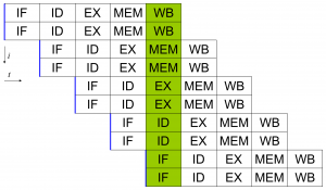
If we look at the pipeline stages above, we can see the following.
addi a0, zero, 10   IF - ID - EXE - MEM - WB
sub  t0, a0, a1          IF - ID* - EXE - MEM - WB
Notice that the value of a0 is not known until stage five (writeback) of the addi instruction. However, the sub instruction needs the value of a0 during its stage two (instruction decode). So, if nothing is done, then the a0 will NOT be zero + 10. It will be whatever was in a0 before the addi instruction.
This is known as a read-after-write data hazard, since the problem is encountered when we try to read a register after it was previously written. This is due to when the register is written.
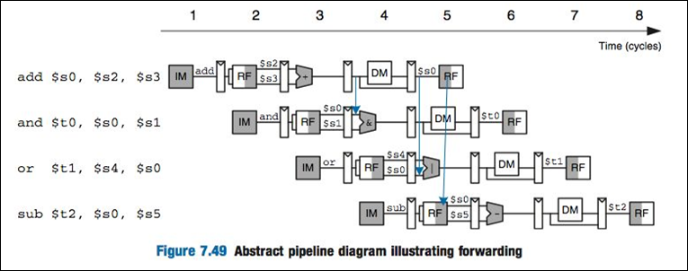
Operand Forwarding
We actually know the value of a0 above after the execute stage of the addi instruction. So, we can forward the output of the execute stage in the addi instruction to the execute stage of the sub instruction. This way, the pipeline can continue without any issues. This technique is known as operand forwarding. Without operand forwarding, we would have to stall the other stages of the sub instruction until the addi instruction had a chance to finish, which would give us the following.
addi a0, zero, 10   IF - ID - EXE - MEM - WB
sub  t0, a0, a1          IF - XXX - XXX - XXX - ID - EXE - MEM - WB
The XXX are known as no operations (nops for short), also known as pipeline stalls, also known as pipeline bubbles. They have no real effect except to wait until the register a0 was written before the sub instruction was executed. We want to avoid pipeline stalls as much as possible. You can see above with all the stalls, the pipeline really has no effect. We might as well run the addi instruction to completion and then execute the sub separately. Thus, this resembles a single-cycle CPU more than it resembles a pipelined CPU.
Structural Hazard
A structural hazard occurs when two or more instructions are ready to use the same functional unit, such as the ALU or register file. These functional units can only operate one at a time, so there is no way to parallelize two instructions. The only real solution to a structural hazard is to add more functional units.
Above shows a two-issue pipeline, where two instructions go through the pipeline simultaneously. In this case, we need an instruction fetcher that’s able to fetch two instructions. We normally see this as a flat model, but think about this in terms of multiple cores. Each core has its own pipeline, decoder, ALU, and so forth. These cores even have their own internal cache. However, the complications come from the MEM stage (or even IF stage) during cache misses.
Control Hazard
Another issue that can arise from pipelining is known as a control hazard, also known as a branch hazard. These arise from branch instruction, such as the following.
here:
   beq a0, a1, there
   add t0, t1, t2
there:
   sub t0, t1, t2
The issue is that until the execute stage, we have no idea whether to fetch the add instruction or the sub instruction. If we load the add instruction and the branch is NOT taken, then there are no issues. However, if we load the add instruction and then the branch is taken, we have to flush the pipeline to remove all remnants of the add instruction.
Branch Prediction
One way to help minimize the effect of branch hazards is to load the most likely instruction. Sometimes a pipeline stall to flush a branch is unavoidable. However, we can use a branch predictor to help predict what is the most likely outcome of a branch instruction.
I will not go into detail on how a branch predictor is designed, but a branch predictor stores the result of every branch up to some limit. When the branch is executed next, the CPU consults the latest branch. If the branch was previously taken, the CPU will load the branch taken. Obviously, just because we took the branch previously doesn’t mean we will again. So, as I mentioned above, flushing the pipeline is not always avoidable.